Energy calibration

X-ray energy calibration using channel-cut crystal

Channel-cut crystal parameters

Length: 36 mm
Width: 3 mm
Lattice spacing (2d): 3.84 Å

Purpose

Calibrate the monochromator energy using the known lattice spacing of the channel-cut crystal.

Procedure

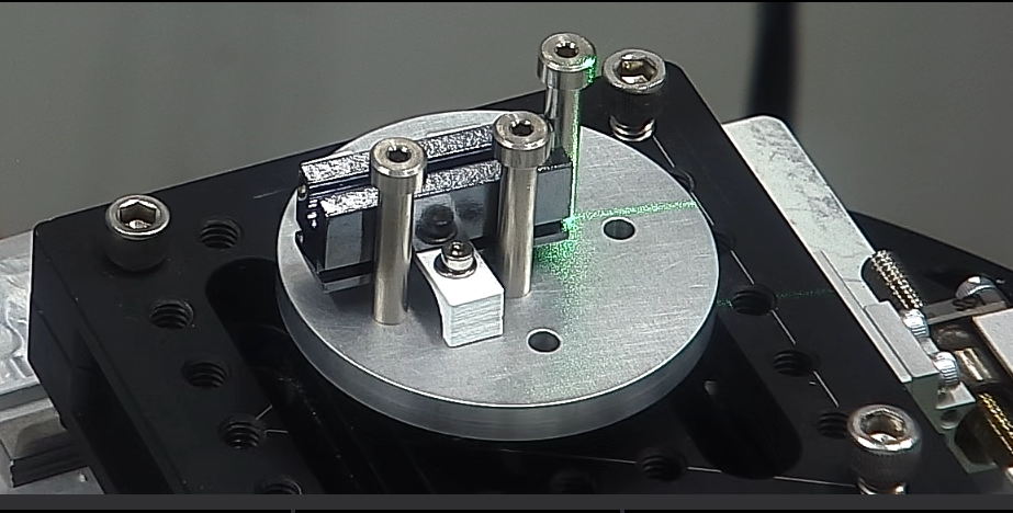
Mount the channel-cut crystal
- Secure the channel-cut crystal on the rotation stage in the x-ray beam path.
- Align the crystal so the incident beam fully illuminates the 3 mm width and the reflection geometry is symmetric.
- Set the rotation angle to zero.
Set initial conditions
- Set the monochromator energy to approximately 20 keV.
- Compute the expected Bragg angle $\theta$ using Bragg’s law:
  
  \[E = \frac{12.3984}{2d \sin\theta} \quad [\text{keV}]\]
  
  Rearranged:
  
  \[\theta = \arcsin\!\left(\frac{12.3984}{2d\,E}\right)\]
  
  where $2d = 3.84\,\text{Å}$ and $E = 20\,\text{keV}$.
- For a 20 keV x-ray beam, the expected Bragg angle is approximately 9.29°.
Example Python code to compute the expected angle:
```
import numpy as np

# Parameters
two_d = 3.84         # 2d in Å
E_nom = 20.0         # nominal energy in keV
hc = 12.3984         # hc in keV·Å

# Compute Bragg angle (radians and degrees)
theta_rad = np.arcsin(hc / (two_d * E_nom))
theta_deg = np.degrees(theta_rad)
print(f"Bragg angle at {E_nom} keV: {theta_deg:.6f}°")
```
Record the reflected x-ray
- Rotate the crystal to the calculated Bragg angle and search for the reflected beam.
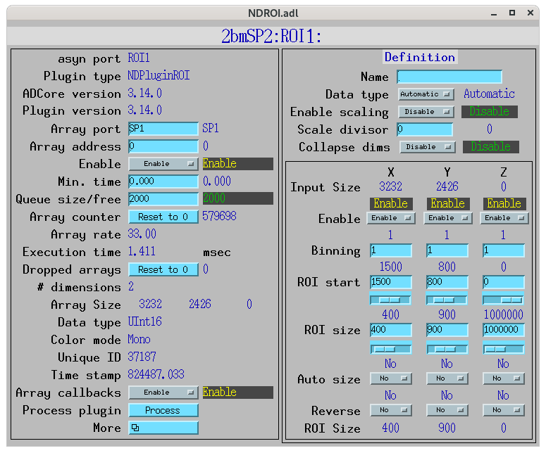
- Select an ROI around the reflection using the ROI plugin in areaDetector.
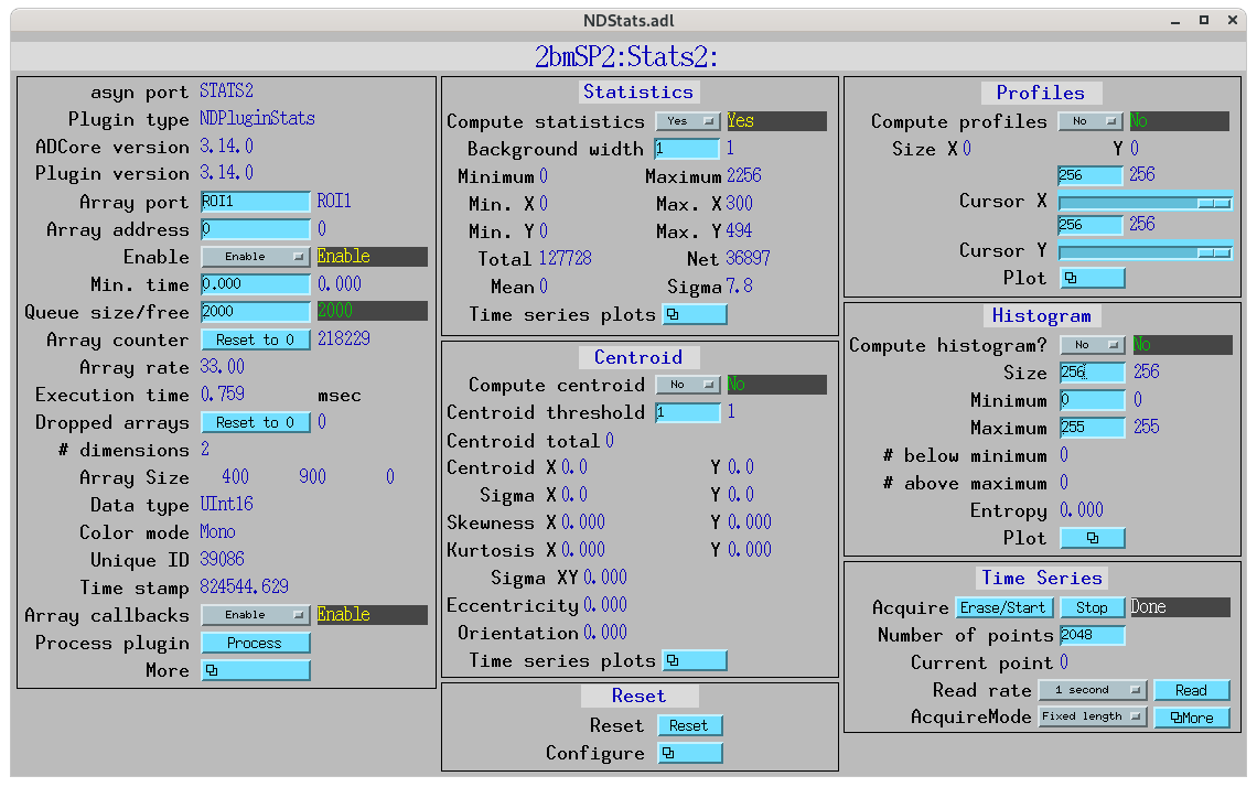
- Use the Stat2 plugin to compute the mean intensity in the ROI.
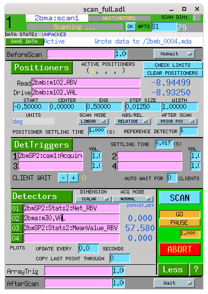
Perform rocking-curve scan
- Perform a fine angular scan (rocking curve) around the calculated Bragg angle to record reflected intensity versus angle.
Identify the peak position
- Fit the rocking curve to determine the Bragg peak angle $\theta_B$.
- $\theta_B$ corresponds to the true Bragg condition at the monochromator setting.
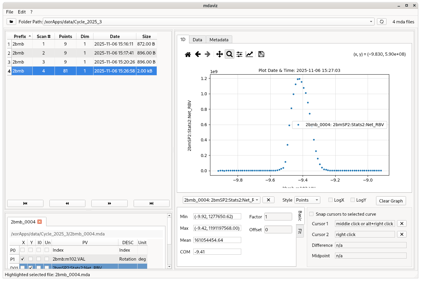
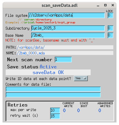
To inspect and fit the data interactively, you can run mdaviz:
```
(base) 2bmb@arcturus $ cd /APSshare/bin
(base) 2bmb@arcturus $ ./mdaviz
```

Calculate the true energy

Compute the actual energy using Bragg’s law:

\[E = \frac{12.3984}{2d \sin\theta_B} \quad [\text{keV}]\]

Example Python code to compute the true energy from the measured peak angle:

import numpy as np

# Parameters
two_d = 3.84         # 2d in Å
E_nom = 20.0         # nominal energy in keV
hc = 12.3984         # hc in keV·Å

# Example: replace with measured peak angle in degrees
theta_B_deg = 9.2903
theta_B_rad = np.radians(theta_B_deg)

# Compute measured energy and offset
E_meas = hc / (two_d * np.sin(theta_B_rad))
offset_keV = E_meas - E_nom

print(f"Measured energy: {E_meas:.6f} keV")
print(f"Offset from nominal: {offset_keV:.6f} keV")

Adjust monochromator calibration
- Compare the calculated true energy to the nominal monochromator value (e.g. 20 keV).
- Apply an energy-offset correction in the control software if required.
Verify calibration
- Repeat the procedure at another energy (e.g. 19 keV or 21 keV) to verify linearity and consistency of the calibration.

Comparison of calculated and measured x-ray energies

The table below lists calculated x-ray energies using a 24 Å W–B₄C multilayer period (first-order Bragg reflection) and compares them with measured energies for various incident angles.

Angle (°)	sin(θ)	λ (Å) = 2d·sinθ	Calculated energy (keV)	Measured energy (keV)
1.1309999999999922	0.0197396	0.9475	13.09	13.374
1.0809999999999933	0.0188718	0.9059	13.68	13.574
0.8220000000000001	0.0143412	0.6884	18.02	18.000
0.726	0.0126695	0.6081	20.39	20.000
0.5772499999999998	0.0100756	0.4836	25.63	25.000
0.5609999999999995	0.0097919	0.4700	26.38	25.584

Note

Calculated energies are obtained from Bragg’s law:

\[E = \frac{12.3984193}{2 d \, \sin\theta} \;\text{[keV]}\]

where $d = 24\,\text{Å}$ is the multilayer period and $\theta$ is the incident angle.

Incident angle for given x-ray energies

The table below shows the incident angle $\theta$ (in degrees) for selected x-ray energies, assuming a 24 Å W–B₄C multilayer and first-order Bragg reflection.

Energy (keV)	Angle °
13	1.145
14	1.061
15	0.990
16	0.928
17	0.872
18	0.823
19	0.779
20	0.739
21	0.703
22	0.670
23	0.640
24	0.612
25	0.586
26	0.561
27	0.538
28	0.517
29	0.497
30	0.478
31	0.460
32	0.443
33	0.426

Note

Angles are in degrees (grazing incidence). They are calculated using Bragg’s law:

\[\theta = \arcsin\left(\frac{12.3984193}{2 d E}\right)\]

where $d = 24\,\text{Å}$ is the multilayer period and $E$ is the desired x-ray energy in keV.